It is a Wild West out there when it comes to testing for attrition in field experiments. Researchers use different tests, describe them with different terms, and somehow always find a way to conclude that attrition is not a problem in their case. So I was happy to read Testing Attrition Bias in Field Experiments by Dalia Ghanem, Sarojini Hirshleifer and Karen Ortiz-Becerra (Journal of Human Resources, 2026; ungated version). It turns out I was doing it wrong. Chances are, so are you.
The authors review 96 published field experiments with baseline data. The most common test — reported in 79 percent of the experiments with attrition above 1 percent — checks whether attrition rates differ between treatment and control. But equal rates are neither necessary for an unbiased estimate nor, without extra assumptions, sufficient: rates can differ while your estimate is fine, and identical rates can hide serious bias. The second most common test, in 61 percent, checks whether treatment and control respondents are balanced at baseline. Closer, but only half of the correct test.
The two tests
To see this, split your baseline sample by treatment status and by endline response:
| Respond | Attrite | |
|---|---|---|
| Treatment | TR | TA |
| Control | CR | CA |
Ghanem and co-authors distinguish two questions:
Test 1: Is the comparison of treatment and control respondents unbiased, for the respondents? The paper calls this internal validity for respondents (IVal-R). The identifying assumption is that treatment is as good as randomly assigned conditional on response status. Its testable implication is that both columns are balanced at baseline, jointly: TR = CR and TA = CA. I used to test each separately.
Test 2: Is that effect also the effect for your original sample? The paper calls this internal validity for the study population (IVal-P). The testable implication is that all four cells are equal. I will call them the respondent test and the representativeness test.
In regression form, using the baseline outcome and the full baseline sample:
Y0 = α + βT Treat + βA Attrite + βTA Treat × Attrite + γ + ε,
where γ are strata fixed effects (more on those below); for clustered designs, standard errors are clustered at the unit of randomization. The respondent test is the joint test βT = βTA = 0. The representativeness test adds one restriction: βA = βT = βTA = 0. Strictly, the paper’s tests compare entire baseline distributions; the regression tests the difference in means, which is what most of us will run, and the two coincide for binary variables.
The authors provide a Stata command that does all of this: ssc install attregtest.
Why also test balance among attritors?
My instinct was that we only care about balance in the sample of respondents, since that is our estimating sample. That is wrong for two reasons. First, the assumption you need, treatment as good as random given response status, has implications for attritors too. Testing respondents only uses half of the testable implications. Second, the respondent-only test is often badly underpowered. Suppose your program keeps some weak students enrolled who would otherwise have dropped out and vanished from the sample. With low attrition, these program-induced responders might be 2 percent of your treatment respondents, far too few to detect in a balance test. But their counterparts in the control group are attritors, where they can be a large proportion of a small group.
What about stratified randomization?
If you randomized within strata, the authors discuss three ways to run the test. The first two work within each stratum, interacting everything with strata dummies: either a single test of all the within-stratum restrictions at once, or a separate test per stratum followed by a multiple-testing correction that controls the family-wise error rate (FWER) or the false discovery rate. The authors motivate the per-stratum version for the case where response problems hit some strata but not others: you stratified by region, say, and one region is remote or flood-prone, so your sample there is hard to reach. The third way is simpler: the regression above, with strata fixed effects and no interactions.
I have two concerns with the within-strata versions.
1. The fully interacted version over-rejects the null, badly so in clustered trials. Interacting the test with strata multiplies the number of restrictions you test at once: with ten strata, the representativeness test already stacks thirty. Tests with many restrictions are known to over-reject when standard errors are clustered (see MacKinnon, Nielsen and Webb 2023 and Kerwin, Rostom and Sterck). I asked Claude to run some simulations (first note at the end; I did not verify the code, but it is consistent with the theory). With 100 clusters, even four strata is too many for the test to hold its size, and with ten strata the within-strata representativeness test rejects 86 percent of the time when nothing is wrong. The same problem arises with heteroskedasticity-robust standard errors under individual-level randomization (Anatolyev and Sølvsten 2023), but there it is far less severe: in the simulations, it only starts to bite once strata fall below roughly 200 observations each.
2. Lower statistical power. Conversely, the fully interacted version has lower power because of its many degrees of freedom, and the FWER correction is conservative. That hands researchers a way to falsely conclude that attrition is not a problem. A second set of simulations (second note at the end), with individual-level randomization so that over-rejection is not the issue, shows that the ranking depends on the nature of attrition. If the attrition problem is diffuse — slight bias in every stratum — the fixed-effects test has the most power and the per-stratum approach with an FWER correction the least. The ranking flips when the violation is concentrated in one stratum, the case the per-stratum approach was designed for.
So I believe it is more sensible to just use the fixed-effects test. The authors agree: they propose it for exactly this situation (Appendix A.2 of the paper, equation 19), use it in their own empirical exercise whenever there are more than ten strata, and attregtest reports both versions. The trade-off is that the fixed-effects version tests an implication of the sharp restriction rather than the restriction itself — a price worth paying once the restrictions pile up.
What about multiple outcomes?
The authors propose that you run the test separately for each endline outcome, using that outcome’s own baseline value and its own response indicator, and correct for multiple testing across outcomes. The paper uses Progresa to show why the per-outcome approach matters, especially if attrition rates vary by outcome. School enrollment fails the representativeness test and adult employment passes it, even though both come from the same survey: households with more school-age children were more likely to skip the enrollment questions.
What if you lack baseline data for an outcome?
Then you test on covariates instead, but not on any covariates. The paper is specific about which ones are admissible: determinants of the outcome, or proxies driven by the same unobservables as the outcome. So pre-specify a small set of outcome-specific determinants, and test them together with the baseline outcome, if you have it, in one system of equations. attregtest takes the whole list and reports one p-value per test for the whole set, as recommended by the authors. At this point the exercise looks a lot like a standard baseline balance table (although it is still run over respondents and attritors on the full baseline sample, not over respondents alone).
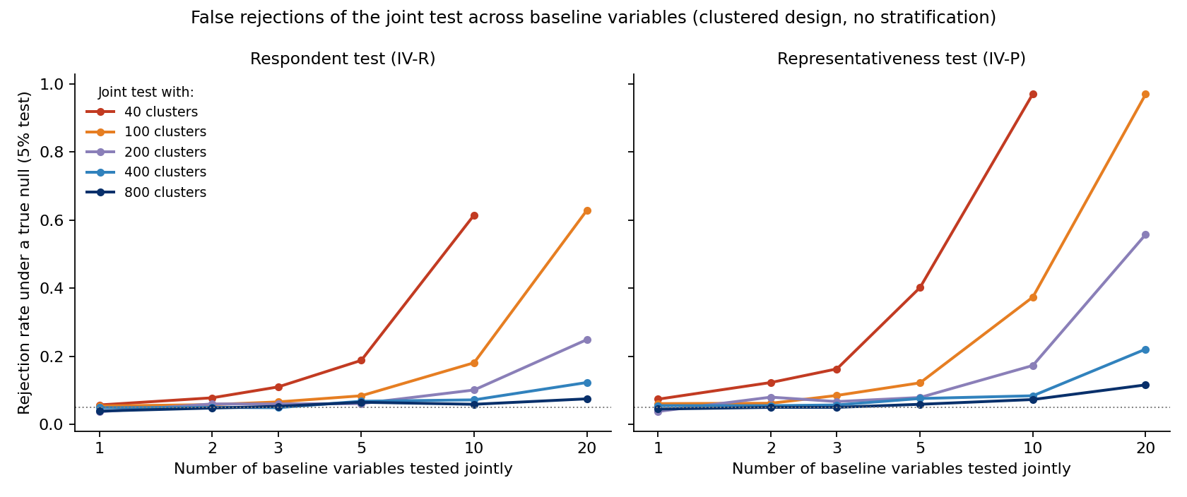
The same warning as above applies, though: with k variables, the respondent test stacks 2k restrictions and the representativeness test 3k, and tests with many restrictions over-reject in clustered designs. In the simulations, with 100 clusters, a representativeness test over ten variables at once falsely rejects 37 percent of the time (first note at the end). If you have more than two or three variables in a clustered design, you need another test. The most viable alternative is to test each variable separately and adjust for multiple tests, using FWER or FDR — for example the sharpened q-values of Anderson (2008). You reject the null if p or q is below your desired level of significance for at least one of the variables. Simulations show that it falsely rejects roughly 7 to 8 percent of the time for a 5 percent test, so it is slightly oversized.
(Aside: my first instinct was to use randomization inference instead, as Kerwin, Rostom and Sterck recommend for balance tests, and as the authors themselves propose in their online appendix for individually randomized experiments. With cluster-level assignment it is not strictly justified, since attrition is itself a post-treatment outcome: re-shuffling schools into treatment and control shuffles their response rates too, so the randomization-inference benchmark implicitly holds attrition unaffected by treatment. In the simulations it does hold its size, but its power is lower than adjusting for multiple tests with Anderson q-values (third note at the end).)
An example from my own work
In our long-run follow-up of the Early Grade Reading Study in South Africa, we found and assessed 67 percent of the treatment group (655 of 981 learners) and 66 percent of the control group (1,035 of 1,575). So attrition was high, but similar across arms. Here are the two tests for three baseline variables:
| Baseline variable | βA | βT | βTA | N | IVal-R | IVal-P |
|---|---|---|---|---|---|---|
| Female | −0.10*** (0.02) | −0.02 (0.02) | 0.02 (0.04) | 2,556 | 0.704 | <0.001 |
| Age | 0.29*** (0.05) | 0.03 (0.05) | −0.07 (0.08) | 2,188 | 0.423 | <0.001 |
| Learning index | −0.21*** (0.06) | 0.08 (0.16) | −0.02 (0.11) | 2,556 | 0.887 | <0.001 |
| All three at once | 2,188 | 0.727 | <0.001 |
Notes: βA is the coefficient on Attrite (the gap between control attritors and control respondents), βT the coefficient on Treat (the treatment–control gap among respondents), and βTA their interaction, from the regression above with strata fixed effects; standard errors, in parentheses, are clustered at the school level, the unit of randomization. The last two columns report p-values from attregtest for the respondent test (IVal-R) and the representativeness test (IVal-P), both in the strata-fixed-effects version. The last row tests all three variables in one system of equations. * p<0.10, ** p<0.05, *** p<0.01.
The respondent (IVal-R) test never rejects, for any variable or for all three at once: treatment and control are balanced within both columns of the two-by-two table. So we cannot reject that our estimate is internally valid for the learners we found, at least for these baseline variables. But the representativeness (IVal-P) test rejects for every variable, and for all three at once: the learners we lost are about a third of a year older, 10 percentage points less likely to be girls, and 0.2 standard deviations weaker on the baseline learning index — and equally so in both arms. Our estimates thus only speak for the two-thirds of the original sample we could still find.
BUT. The within-strata version of the test tells a different story: it rejects the respondent test for the learning index (p = 0.004) and for all three variables at once (p < 0.001). Had we quoted those numbers, we would have concluded that the study is not internally valid even for respondents. But this is exactly the fragile test from my first concern above: with ten strata and 130 schools, the fully interacted within-strata test stacks 60 (10 × 3 × 2) restrictions on 130 clusters — and even the single-variable version stacks 20. The simulations say such tests reject many times too often under a true null.
The bottom line
Report attrition rates by arm with their cell sizes, but as a description of the response process, not as a test of validity. Report the four cell means and the two joint p-values, per outcome, from one regression on data you already have. Pre-specify the variables and, if you stratified, the version of the test — and in a clustered design with many strata or many variables, that version should be the fixed-effects one. If you have many baseline variables in a clustered design, test them one at a time with a multiple-testing correction. If the representativeness test fails, say plainly which population your estimate covers. If the respondent test fails, no test will rescue you: you are in the territory of attrition corrections and bounds.
Simulation note 1: tests with many restrictions in clustered designs
A cluster-randomized experiment with G schools of 20 learners, half of the schools in each stratum treated, 30 percent attrition unrelated to anything, and one baseline variable that is pure noise (intra-cluster correlation 0.15). Both tests should therefore reject 5 percent of the time. The tests are the standard regression tests as Stata computes them (cluster-robust standard errors, F critical values with G − 1 denominator degrees of freedom), in two versions: the strata-fixed-effects regression in the post, and the fully interacted within-strata version, whose restriction count grows with the number of strata (2S for the respondent test, 3S for the representativeness test). One thousand replications per cell.
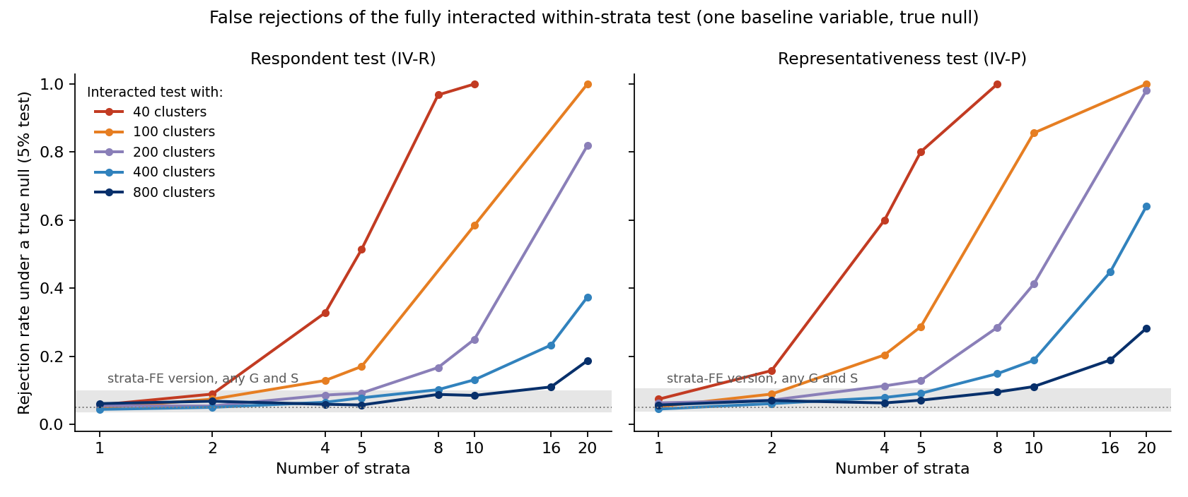
The fixed-effects version approximately holds its size everywhere: 4 to 10 percent for every combination of strata and clusters (the gray band). The within-strata version deteriorates as restrictions accumulate relative to clusters. With 100 clusters: at two strata the representativeness test falsely rejects 9 percent of the time, at four strata 20 percent, at ten strata 86 percent, and at twenty strata always. Even 400 clusters are not safe at ten strata (19 percent). In the extreme — two treated clusters per stratum — the within-stratum representativeness test is not even defined, and Stata silently drops constraints.
The problem compounds when multiple baseline variables are tested at once. With k variables, the respondent test has 2 × k restrictions and the representativeness test 3 × k; the within-strata versions multiply both by the number of strata. The next figure repeats the exercise in an unstratified design, varying the number of variables and the number of clusters (variables correlated at 0.3), and the trajectory is the same: with 100 clusters, a representativeness test over ten variables at once falsely rejects 37 percent of the time, and over twenty variables 97 percent. At the same number of restrictions, the strata version is worse — a within-stratum comparison draws only on the clusters in that stratum, while a variable’s restrictions draw on all of them — but the practical rule is identical: keep the number of restrictions small relative to the number of clusters.
The same exercise with individual-level randomization and heteroskedasticity-robust standard errors (the outcome variance differs across strata) shows the same pattern in a much milder form. Size stays near 5 percent unless strata become small: with 2,000 observations the tests are close to nominal through ten strata, but with 800 observations and 16 strata the representativeness test rejects 36 percent of the time, and at 20 strata it frequently cannot be computed at all.
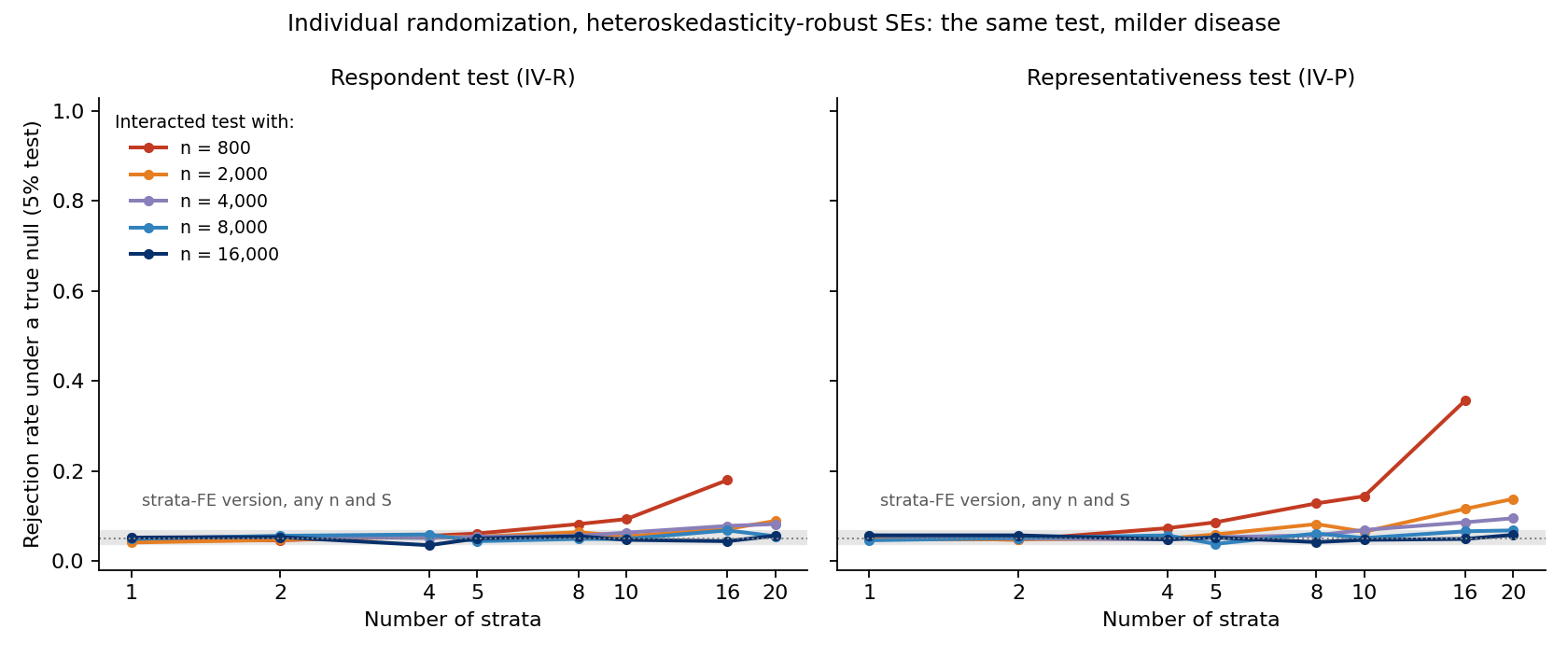
Design caveats for these exercises: equal-sized strata, and variables correlated at 0.3 in the many-variables case.
Simulation note 2: joint versus per-stratum tests
A stratified experiment with 10 strata of 200 units (n = 2,000), treatment assigned at the individual level within strata, a baseline outcome with a standard deviation of 15, and 10 percent never-responders. The respondent assumption is violated by adding treatment-only responders (10 percent of the sample) with a lower baseline mean, which contaminates both columns of the two-by-two table. Two geometries with the same total signal: concentrated, where the whole violation sits in one stratum, and diffuse, where it is spread evenly over all ten. Four tests of the respondent null, all regression-based: the fixed-effects regression in the post (2 restrictions); the fully interacted test across strata (20 restrictions); and per-stratum tests with a Bonferroni–Holm or a Benjamini–Hochberg correction. With individual-level assignment, all four hold size at 5 percent — the clustering problem from the first note does not arise. Power at a total violation of 30 baseline points, or two standard deviations (3,000 replications):
| Geometry | Fixed effects | Fully interacted, all strata | Per-stratum + FWER | Per-stratum + FDR |
|---|---|---|---|---|
| Diffuse (all 10 strata) | 0.74 | 0.33 | 0.18 | 0.19 |
| Concentrated (1 of 10) | 0.14 | 0.33 | 0.46 | 0.47 |
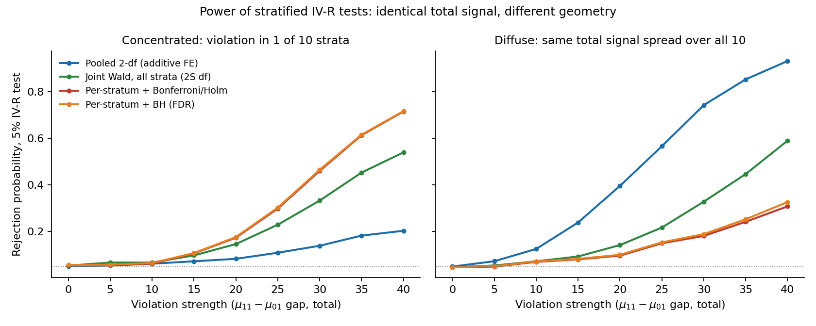
Caveats: individual-level randomization only, mean tests only, equal-sized strata.
Simulation note 3: testing multiple variables in clustered designs
Setup: 100 schools of 20 learners in ten strata, half of the schools in each stratum treated; k baseline variables (3 or 10), correlated at 0.3 across variables; all statistics are strata-fixed-effects regression tests with clustered standard errors. Attrition is caused by treatment: 60 percent of learners respond in control schools and 70 percent in treated schools — a demanding case for randomization inference, since attrition is a post-treatment outcome. Under the null, attritors are otherwise identical to respondents. Two violations of the same total size: a concentrated one, where learners who respond only when treated score 0.5 standard deviations lower on one variable, and a diffuse one, where they score 0.5/√k lower on every variable. Three ways of testing the k variables: one at a time with Anderson-style sharpened q-values across variables, rejecting if any q-value falls below 0.05; all at once in one system with F critical values; and the same system test with randomization inference, which re-assigns treatment across schools within strata and recomputes the statistic 199 times. Four hundred replications.
| Size under the null | Power: violation in one variable | Power: violation in all variables | |
|---|---|---|---|
| Per variable + sharpened q-values | 0.07–0.08 | 0.21–0.34 | 0.12–0.25 |
| All variables at once + randomization inference | 0.05–0.07 | 0.16–0.31 | 0.08–0.19 |
| All variables at once, F critical values | 0.08–0.46 | — | — |
Notes: each cell is a rejection rate for a 5 percent test. Size is the rejection rate when nothing is wrong, so 0.05 is correct and anything higher means the test over-rejects; power is the rejection rate under the violation, where higher is better. No power is reported for the all-at-once test with F critical values, since rejection rates say nothing about a test whose size reaches 0.46. The two violations have shifts of the same total length, but spreading a shift across correlated variables makes it harder for any test to detect, so the two power columns are comparable across rows and not with each other. Each range spans the two tests (respondent and representativeness) and the two list lengths (k = 3 and k = 10); the longer list gives the worse size and the lower power in every row. Monte Carlo error is roughly ±0.015.
References
Anatolyev, Stanislav, and Mikkel Sølvsten. 2023. “Testing Many Restrictions Under Heteroskedasticity.” Journal of Econometrics 236(1), 105473. [journal] [ungated]
Anderson, Michael L. 2008. “Multiple Inference and Gender Differences in the Effects of Early Intervention: A Reevaluation of the Abecedarian, Perry Preschool, and Early Training Projects.” Journal of the American Statistical Association 103(484): 1481–1495. [link]
Cilliers, Jacobus, Brahm Fleisch, Cas Prinsloo and Stephen Taylor. 2020. “How to Improve Teaching Practice? An Experimental Comparison of Centralized Training and In-Classroom Coaching.” Journal of Human Resources 55(3): 926–962. [link]
Ghanem, Dalia, Sarojini Hirshleifer and Karen Ortiz-Becerra. 2026. “Testing Attrition Bias in Field Experiments.” Journal of Human Resources 61(2): 690–731. [journal] [ungated] [online appendix]
Ghanem, Dalia, Sarojini Hirshleifer and Karen Ortiz-Becerra. “attregtest: Stata module to implement regression-based attrition tests.” Statistical Software Components, Boston College. Install with ssc install attregtest. [link]
Kerwin, Jason, Nada Rostom and Olivier Sterck. 2024. “Striking the Right Balance: Why Standard Balance Tests Over-Reject the Null, and How to Fix It.” IZA Discussion Paper 17217. [link]
Lee, David S. 2009. “Training, Wages, and Sample Selection: Estimating Sharp Bounds on Treatment Effects.” Review of Economic Studies 76(3): 1071–1102. [link]
MacKinnon, James G., Morten Ørregaard Nielsen and Matthew D. Webb. 2023. “Cluster-Robust Inference: A Guide to Empirical Practice.” Journal of Econometrics 232(2): 272–299. [link]